Departmental Performance Management

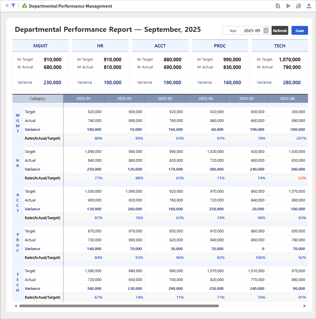
This report enables real-time consolidation and management of departmental performance data on the web.

Move beyond the hassle of collecting data in Excel — now manage all performance records in one integrated online view.

Easily consolidate target, actual, variance, and achievement rate data for each department, giving managers instant visibility into overall performance without manual updates.

Use the provided sample Excel file to experience a more efficient way to manage departmental performance.

Step 1. Convert an Excel file to a web report using i-AUD Designer

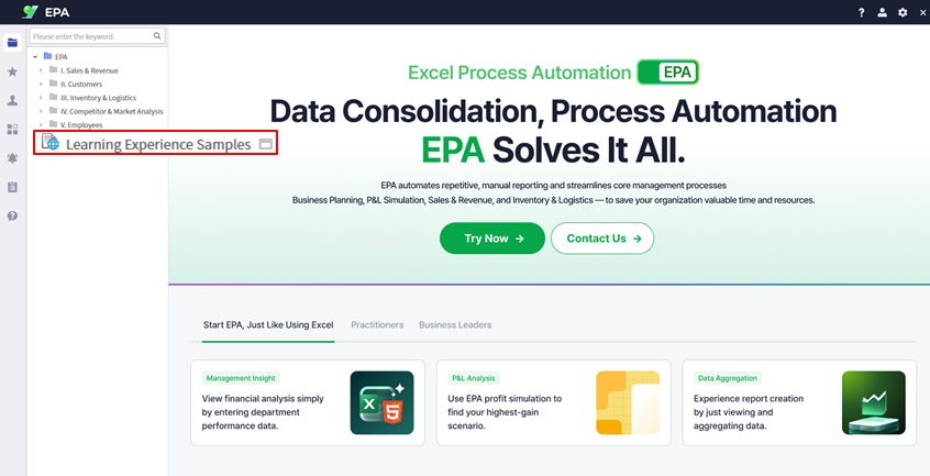
1. • Download the sample Excel file from the Learning Experience Samples.
     
     
     

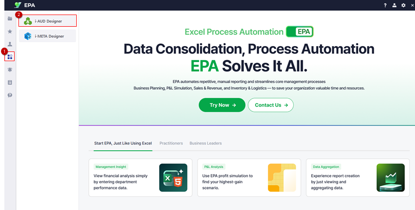
   • From the EPA main screen, go to [Menu] > [Tool] and launch i-AUD Designer.
     
     
     

   • Drag and drop the saved Excel file into the i-AUD Designer window.
     
     
     
     

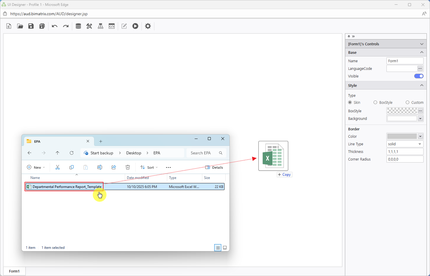
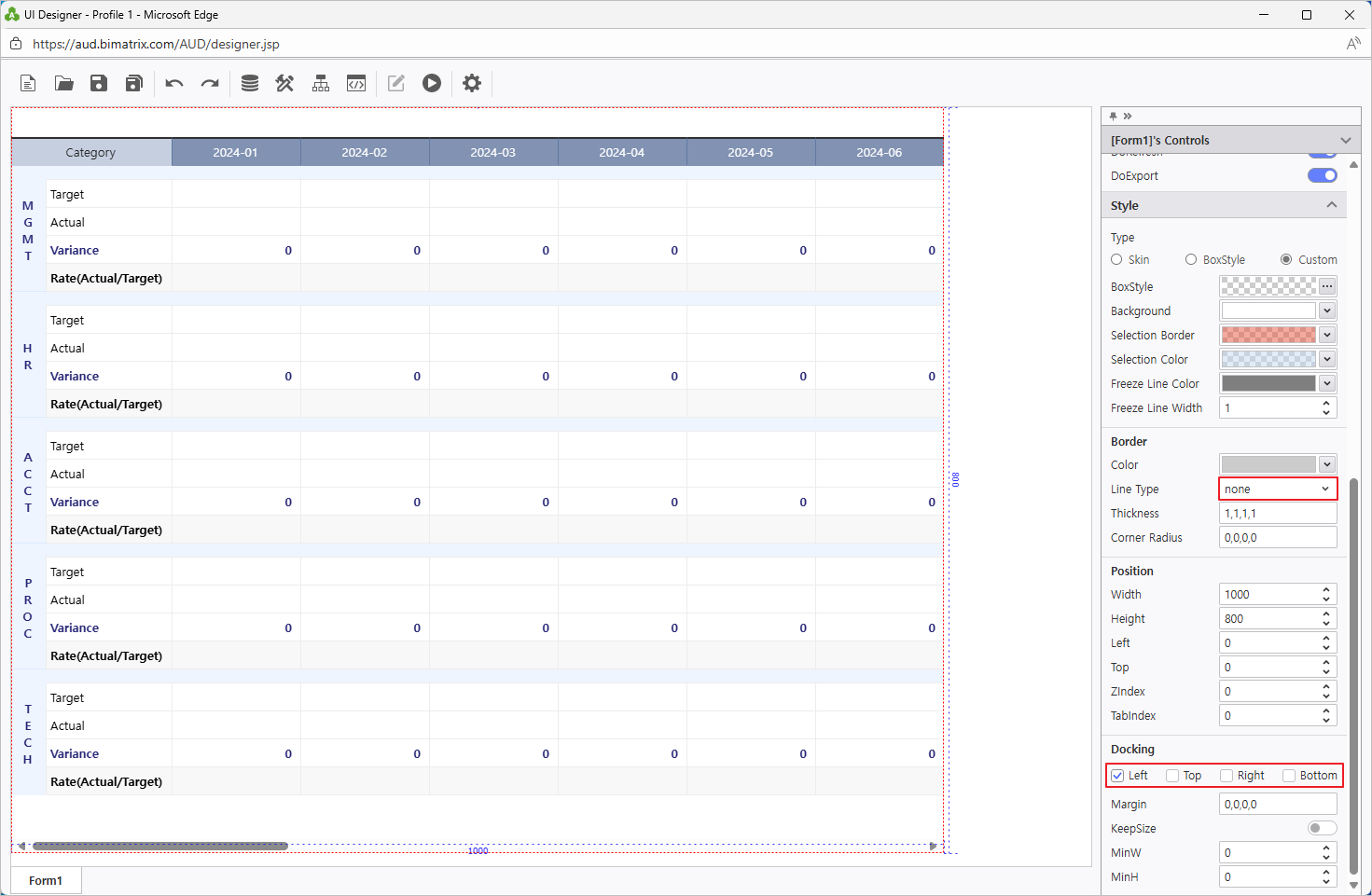
   • Ensure the report automatically resizes to fit the web browser window.

   • In the Properties pane on the right, check Docking: Left.

   • To remove the border from the report on the designer screen, set the Line Type property under Border to ‘None’.
     
     

Step 2. Configure the data input screen

• • Using Excel’s ‘Name Manager’ and the UI Bot, set up the report so that data can be entered directly on the web. 

  • Right-click on the report area, then select Design.

    Naming Rules for the Data Input Screen

    To configure the data input screen, you must follow these three rules:

    1. Name the data entry area “data1”.
       Set the cell format to ‘Number’ for numeric input and ‘Text’ for text input.
       
       

    2. Name the table area to be aggregated “table1”.
       
       

    3. In the top-left corner of the area defined as table1, you must enter the table name.
       

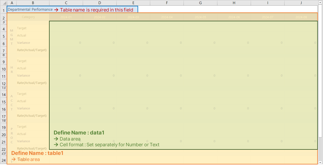
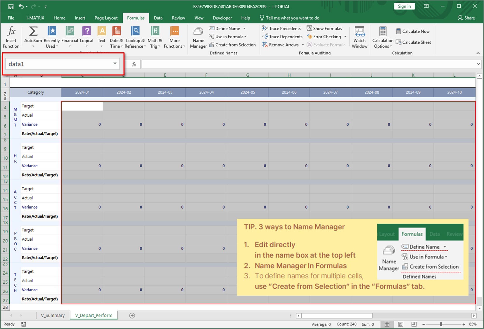
  • According to the rules, select the area on the sheet where data will be entered and name it “data1”.
    
    
    

  • Select the entire table form to be aggregated and name it “table1”.
    
    
    

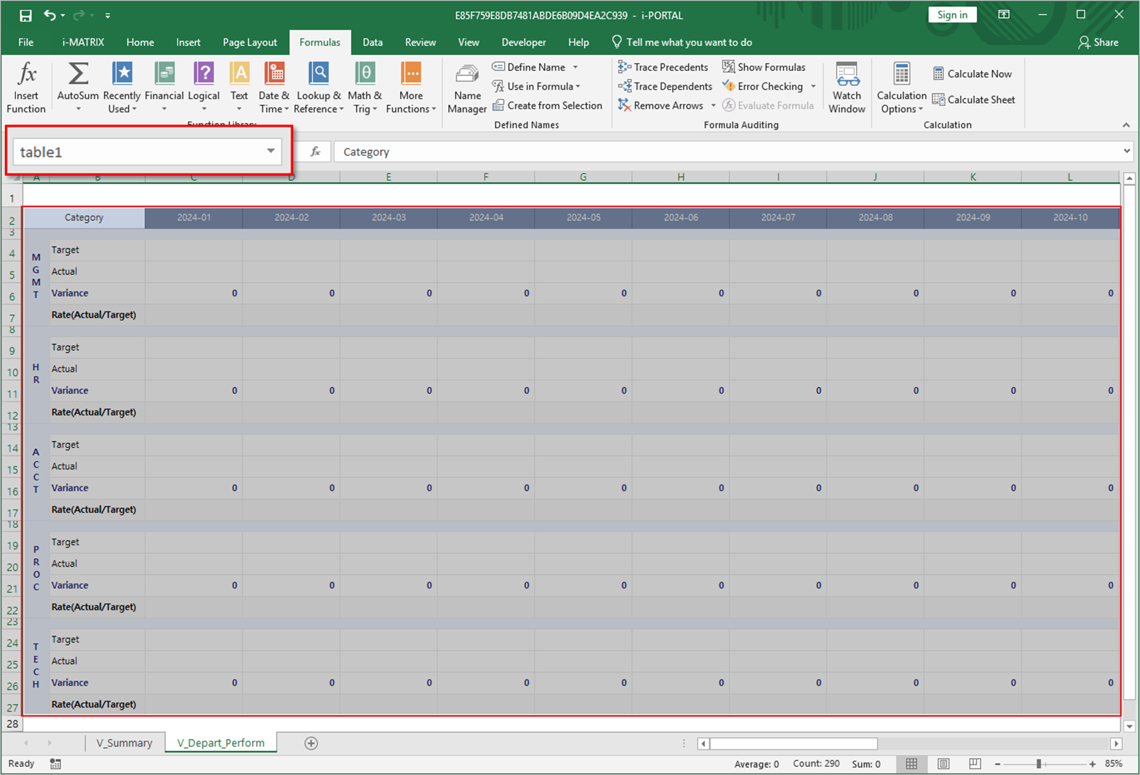
  • In the top-left corner of the area defined as table1, enter the table name.
    If you don’t want this to be visible on the web, you can hide the row in Excel.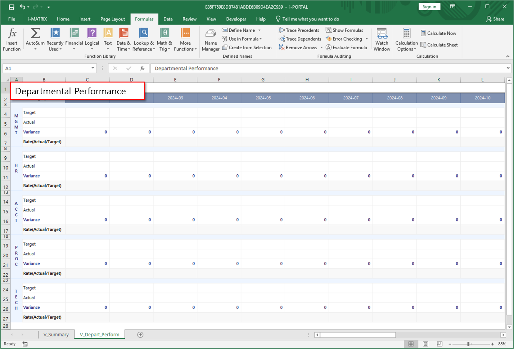
    
    
    
  • The setup for web data entry is now complete.
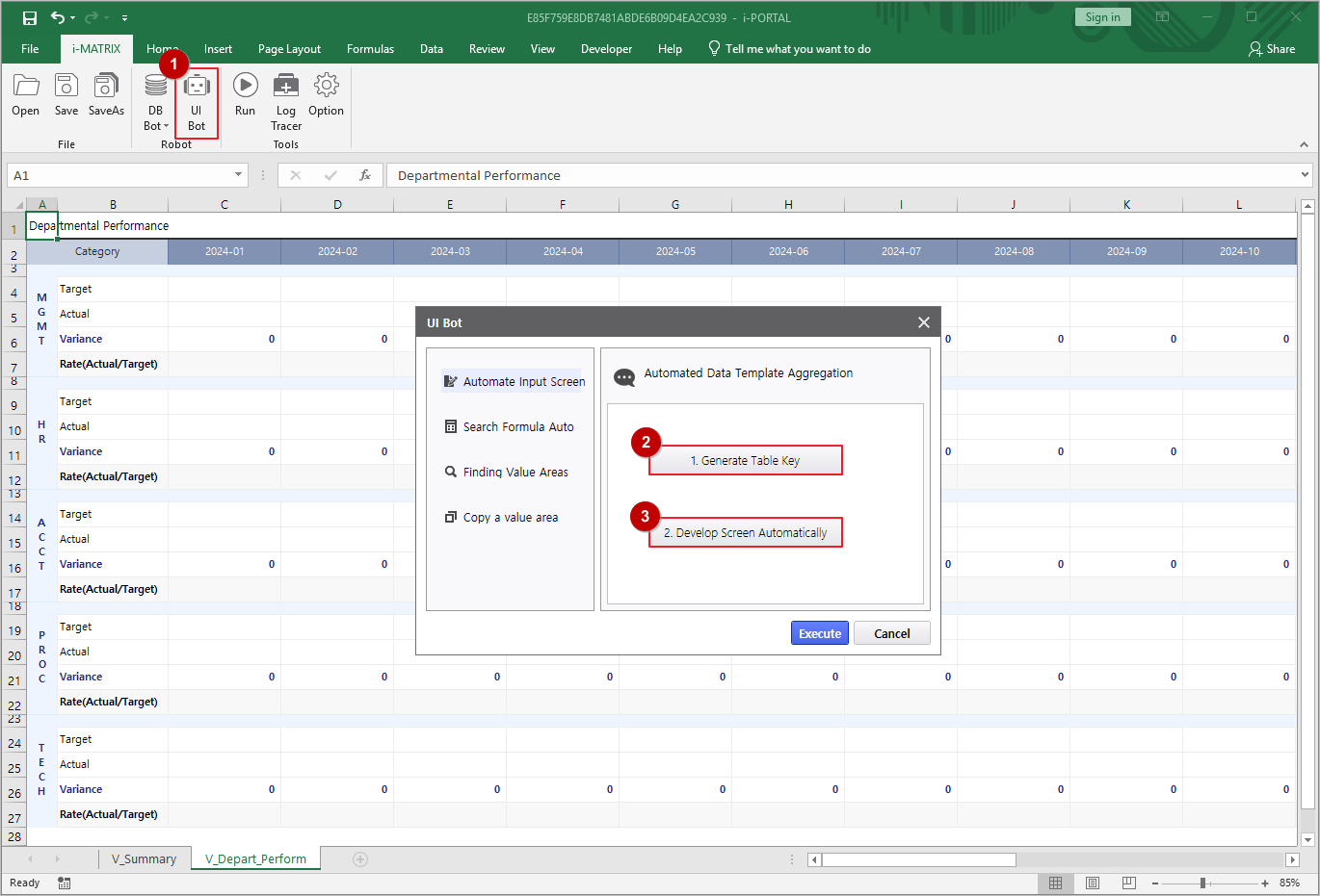
    Next, we will configure the report so that data can be entered and saved with a click, and the saved data can be retrieved.
    
    

  • Go to the ‘i-MATRIX’ tab in the ribbon and click 'UI Bot’.
    
    
    
    

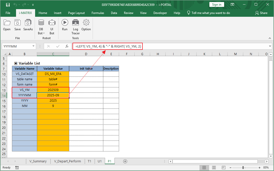
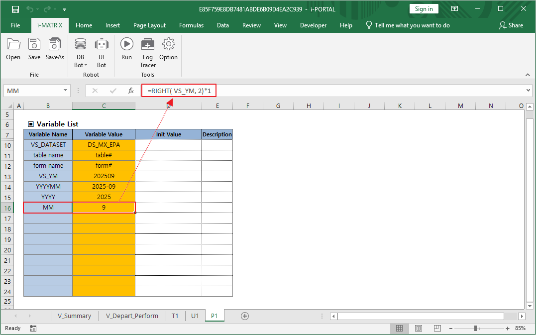
  • Move to the P1 sheet. Use the VS_YM variable so that department performance can be displayed based on the date selected via the calendar.
  • Define the VS_YM variable and enter the desired year and month.
  • Additionally, define YYYYMM, YYYY, and MM, and set the formulas as follows.
    
    
  • YYYYMM formula : =LEFT( VS_YM, 4) & "-" & RIGHT( VS_YM, 2)
    
    
    
  • YYYY formula : =LEFT( VS_YM,  4)*1
    
    
    
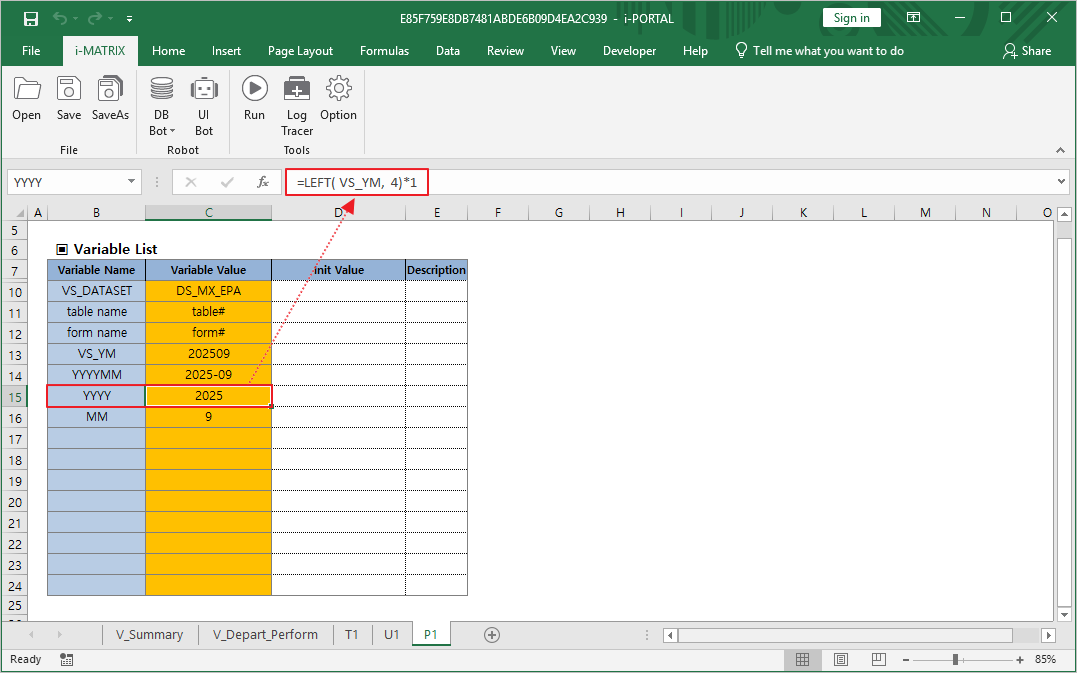
  • MM formula : =RIGHT( VS_YM, 2)*1
    
    
    
  • Now, let’s move to the ‘V_Depart_Perform’ sheet.
  • Use AUD_HIDE_COLUMNS to hide columns in the web display that fall outside the selected year and month.
    Formula : =AUD_HIDE_COLUMNS( OR(  LEFT( E4, 4 )*1 <>  YYYY,  RIGHT( E4, 2 )*1 > MM  ))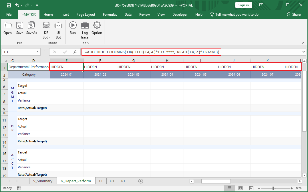
    
    
    
  • On the ‘V_Summary’ sheet, display the data entry screen title in the top-left corner.
    Formula : ="Departmental Performance Report — " & TEXT(DATE(LEFT(VS_YM, 4), RIGHT(VS_YM, 2), 1), "mmmm") & ", " & YYYY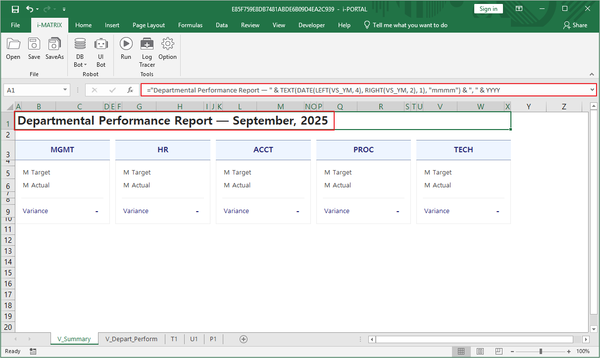
    
    
    
  • The report setup and save are now complete. Return to the i-AUD Designer screen.

Step 3. Connect to the DB for data storage and configure buttons

• • In AUD Designer, double-click an empty cell in the data area and enter a number. Verify that the value is entered and totals are calculated automatically.

  • To save the entered data to the database, connect to the DB and configure the Save and Retrieve buttons.
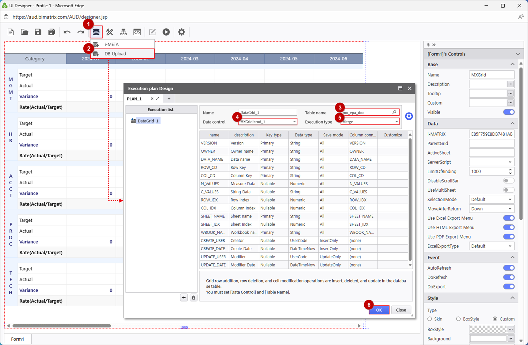
  • Go to DB Bot > DB Upload and register an execution plan.
  • Enter the ‘Table Name’ and select the ‘Data Control’ containing the data to be saved. Then, columns will be automatically mapped.
  • Set ‘Execution Type’ to ‘Merge’.
    
    
    
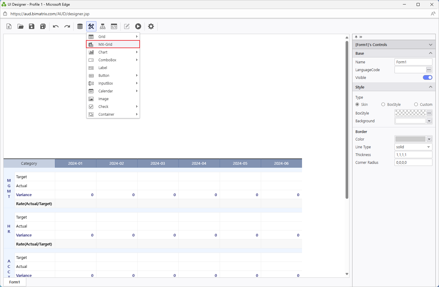
  • To display different V sheets in a single MXGrid, add a new MXGrid from UI Bot > MXGrid.
    
    
    
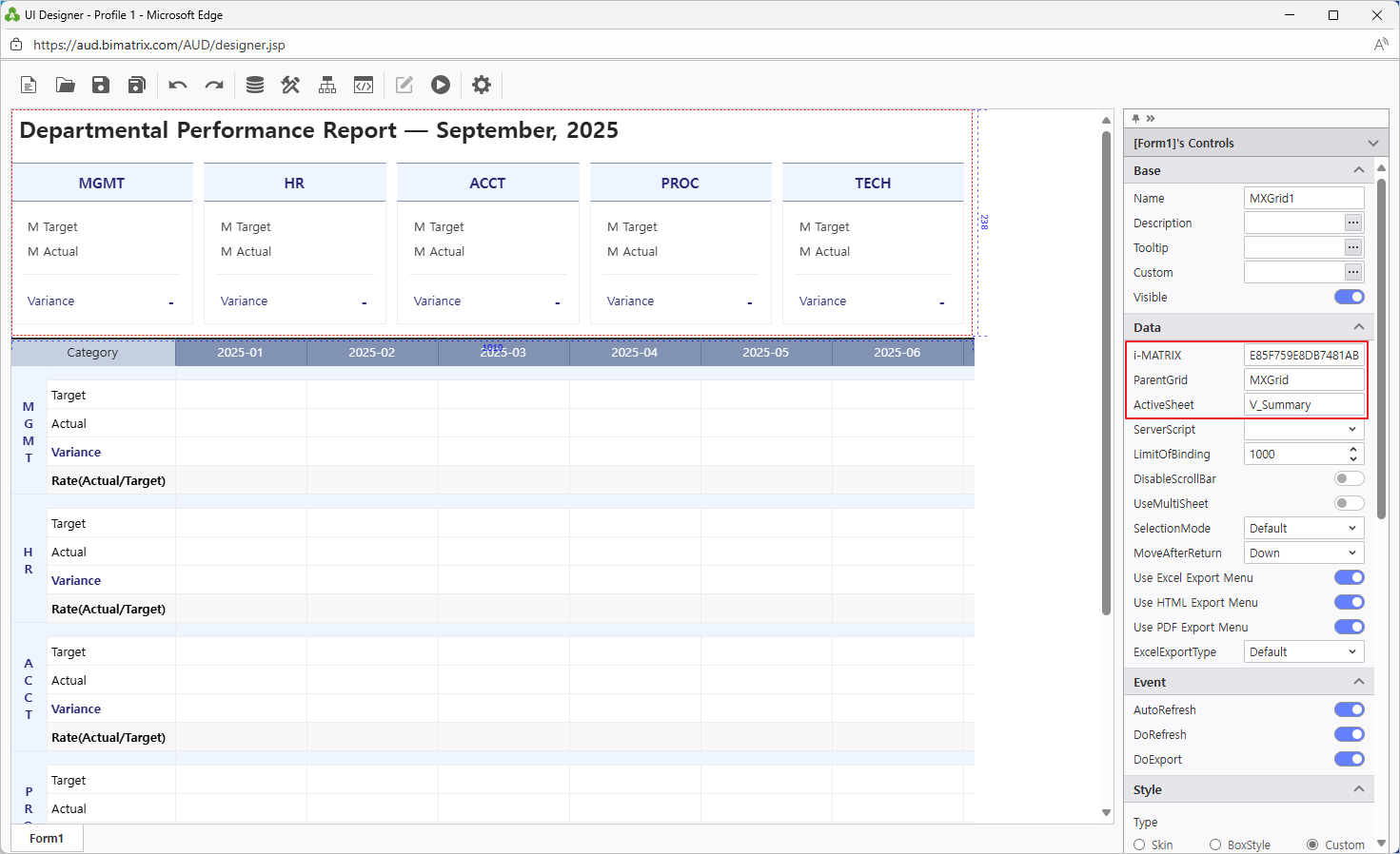
  • Copy the code entered in the i-MATRIX property under Data of the previously placed ‘MXGrid’ and paste it into the same location for the newly added ‘MXGrid1’.
  • Set ‘ParentGrid’ to the name of the first MXGrid.
  • Set ActiveSheet to the sheet you want to display. Enter ‘V_Summary’ to new MXGrid1.
    
    
    
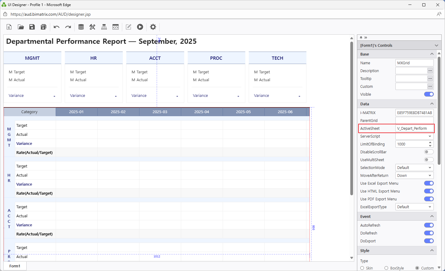
  • Enter ‘V_Depart_Perform’ to previously placed MXGrid.
    
    
    
  • The setup for saving data is complete.
  • Now, let's save the entered data to the DB and set up a button to retrieve the saved data.
    
    
  • Add two buttons from UI Bot > Button and place them in appropriate positions.
  • Rename the buttons to distinguish their functions.
    'Save' : BTN_SAVE
    'Refresh' : BTN_REFRESH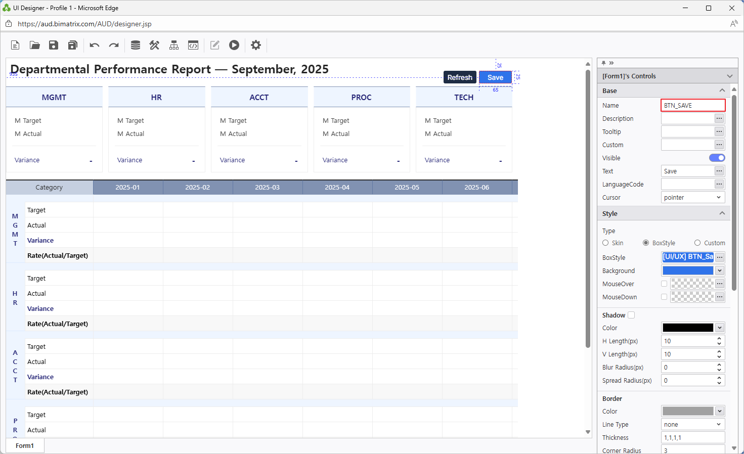
    
    
    
  • Use Process Bot to assign actions to the buttons.
    
    
    
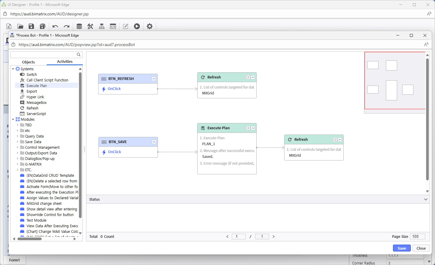
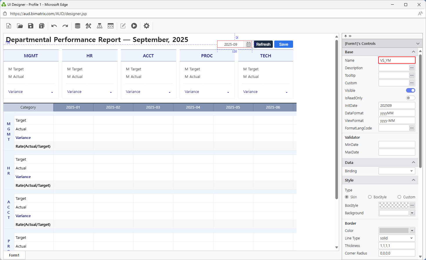
  • Add a year-month calendar using UI Bot > Calendar > Month.
    
  • Link it to the Excel named cell by setting Name to VS_YM so that data can be retrieved based on the selected month.
    
    
    
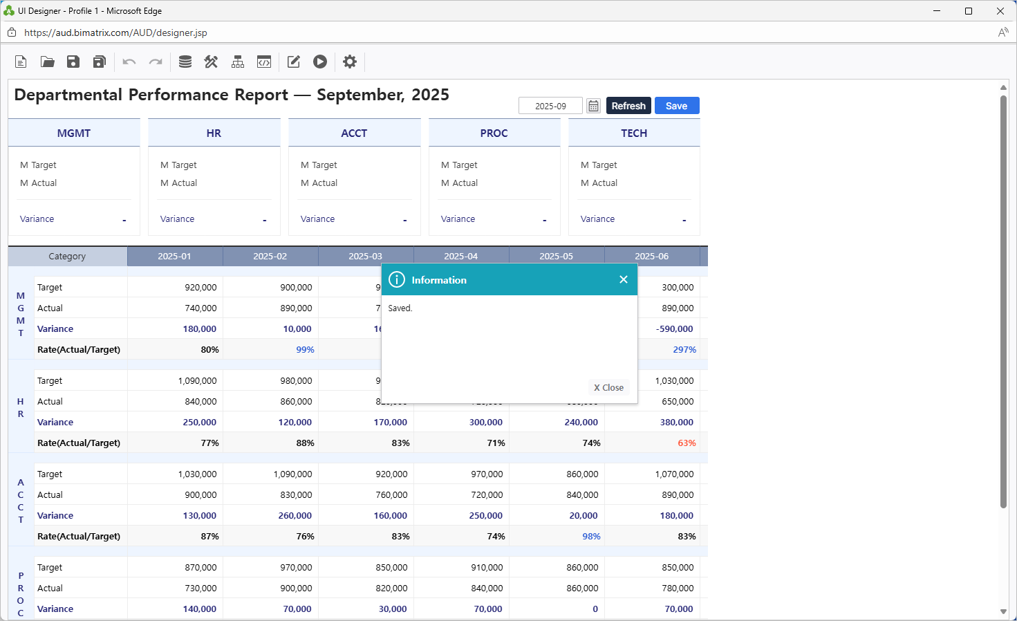
  • Once this is set up, entering data and clicking the ‘Save’ button will store the data in the database, and the 'Refresh' button will fetch the stored data.
    
    

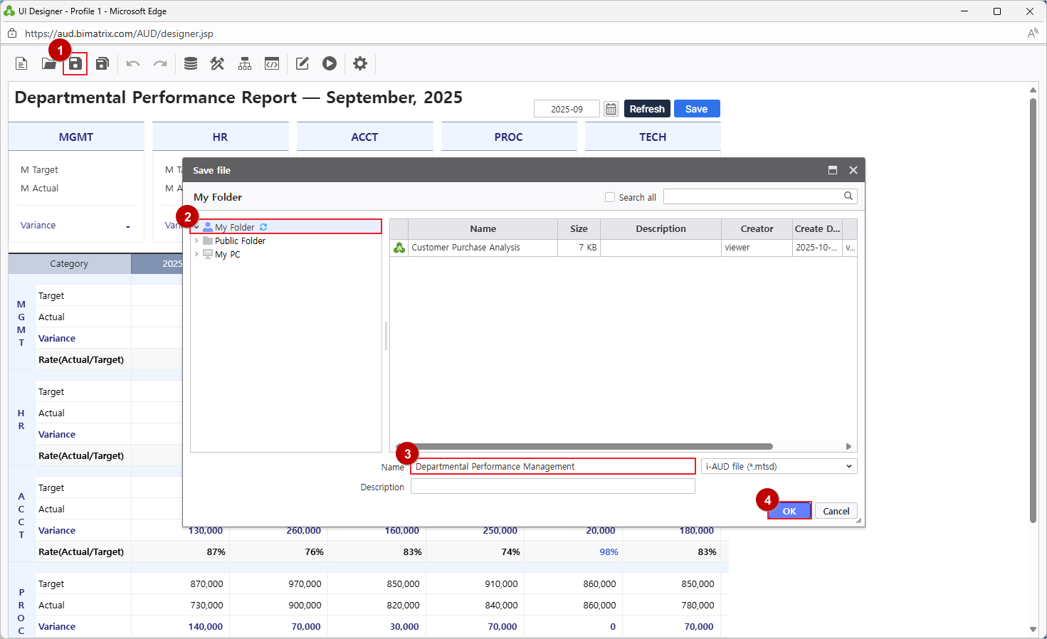
Step 4. Save your report

• • Save the completed report to My Folder.
    
    
    

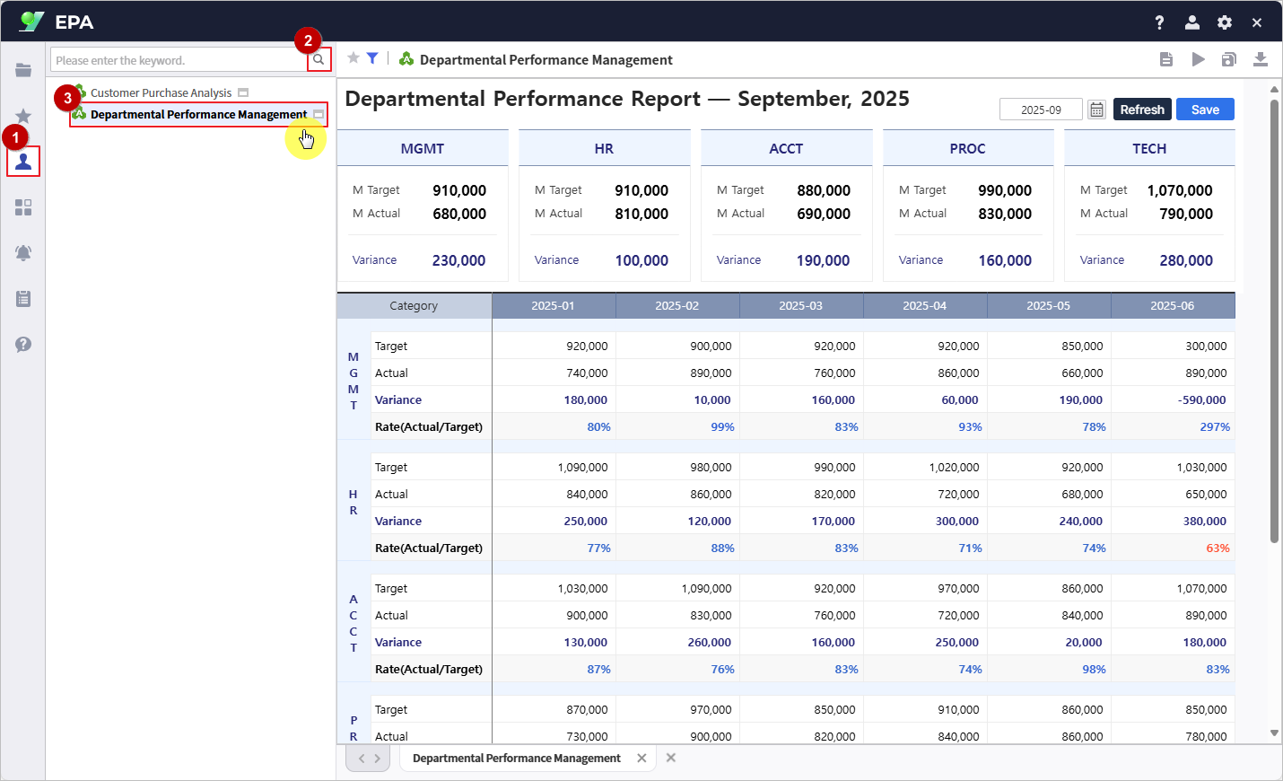
  • From the EPA main screen, go to [Menu] > [Individual] in the left-hand sidebar.

  • Click the Search(Magnifying glass icon) button to refresh the report list and confirm your saved report.

  • Enter data on the web and save it to share with your team.